This is adapted from harvard AnnotatedTransformer, which gives an annotated implementation of the Transformer model from the paper “Attention is All You Need” (Vaswani et al., 2017). The original code can be found at https://nlp.seas.harvard.edu/annotated-transformer/.
import os from os.path import exists import torch import torch.nn as nn from torch.nn.functional import log_softmax, pad import math import copy import time from torch.optim.lr_scheduler import LambdaLR import pandas as pd import altair as alt from torchtext.data.functional import to_map_style_dataset from torch.utils.data import DataLoader from torchtext.vocab import build_vocab_from_iterator import torchtext.datasets as datasets import spacy import GPUtil import warnings from torch.utils.data.distributed import DistributedSampler import torch.distributed as dist import torch.multiprocessing as mp from torch.nn.parallel import DistributedDataParallel as DDP
# Set to False to skip notebook execution (e.g. for debugging) warnings.filterwarnings("ignore") RUN_EXAMPLES = True
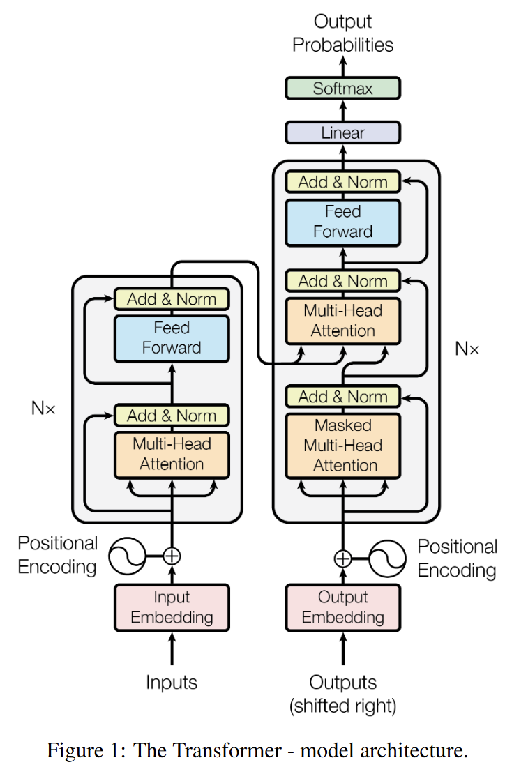
Most competitive neural sequence transduction models have an encoder-decoder structure.
Here, the encoder maps an input sequence of symbol representations \((x_1, ..., x_n)\) to a sequence of continuous representations \(z = (z_1, ..., z_n)\). Given \(z\), the decoder then generates an output sequence \((y_1, ..., y_m)\) of symbols one element at a time. At each step the model is auto-regressive, consuming the previously generated symbols as additional input when generating the next.
# Most competitive neural sequence transduction models have an encoder-decoder structure [5, 2, 35]. # Here, the encoder maps an input sequence of symbol representations (x1, ..., xn) to a sequence # of continuous representations z = (z1, ..., zn). Given z, the decoder then generates an output # sequence (y1, ..., ym) of symbols one element at a time. At each step the model is auto-regressive # [10], consuming the previously generated symbols as additional input when generating the next.
classEncoderDecoder(nn.Module): # Corresponds to the Encoder-Decoder architecture in the figure above. """ A standard Encoder-Decoder architecture. Base for this and many other models. """ def__init__(self, encoder, decoder, source_embed, target_embed, generator): super(EncoderDecoder, self).__init__() self.encoder = encoder self.decoder = decoder self.source_embed = source_embed # See Embedding and Softmax Part self.target_embed = target_embed self.generator = generator defforward(self, source, target, source_mask, target_mask): "Take in and process masked source and target sequences" returnself.decode(self.encode(source, source_mask), source_mask, target, target_mask) defencode(self, source, source_mask): returnself.encoder(self.source_embed(source), source_mask) defdecode(self, memory, source_mask, target, target_mask): returnself.decoder(self.target_embed(target), memory, source_mask, target_mask) # data type: # source, source_mask: (batch_size, source_seq_len) # target, target_mask: (batch_size, target_seq_len) # source_embed: (batch_size, source_seq_len, d_model), embedding of source sequence # target_embed: (batch_size, target_seq_len, d_model), embedding of target sequence # generator: (batch_size, target_seq_len, vocab_size), output of the model classGenerator(nn.Module): # Corresponds to the top two layers in the figure above. "Standard Linear + Softmax generation step, output probabilities" def__init__(self, d_model, vocab_size): super(Generator, self).__init__() self.proj = nn.Linear(d_model, vocab_size) defforward(self, x): return log_softmax(self.proj(x), dim=-1)
Encoder and Decoder Stacks
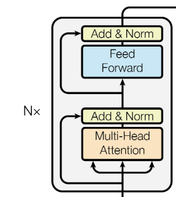
Encoder: The encoder is composed of a stack of \(N=6\) identical layers. Each layer has two sub-layers. The first is a multi-head self-attention mechanism, and the second is a simple, position-wise fully connected feed-forward network.
We employ a residual connection around each of the two sub-layers, followed by layer normalization [1]. That is, the output of each sub-layer is \(\text{LayerNorm}(x + \text{Sublayer}(x))\), where \(\text{Sublayer}(x)\) is the function implemented by the sub-layer itself.
To facilitate these residual connections, all sub-layers in the model produce outputs of dimension \(d_{model} = 512\).
LayerNorm normalizes across the features, while BatchNorm normalizes across the batch dimension.
LayerNorm is more suitable for RNNs and Transformers, where the batch size can vary or be small.
Self-Attention: use lambda x: self.self_attn(x, x, x, mask) because in self-attention, \(Q,K,V\) all come from \(x\), while in cross-attention, \(Q\) comes from the decoder’s previous layer output, and \(K,V\) come from the encoder’s output.
classLayerNorm(nn.Module): "Construct a layernorm module (See citation for details)." # Corresponds to the "Add & Norm" part in the figure above. def__init__(self, features, eps=1e-6): self.a = nn.Parameter(torch.ones(features)) self.b = nn.Parameter(torch.zeros(features)) self.eps = eps defforward(self, x): mean = x.mean(-1, keepdim=True) std = x.std(-1, keepdim=True) returnself.a * (x - mean) / (std + self.eps) + self.b
defclones(module, N): "Produce N identical layers." return nn.ModuleList([copy.deepcopy(module) for _ inrange(N)])
classEncoder(nn.Module): "Core encoder is a stack of N layers, but layer is not defined here" def__init__(self, layer, N): super(Encoder, self).__init__() self.layers = clones(layer, N) self.norm = LayerNorm(layer.size) defforward(self, x, mask): for layer inself.layers: x = layer(x, mask) returnself.norm(x)
classSublayerConnection(nn.Module): """ A residual connection followed by a layer norm Note for code simplicity the norm is first as opposed to last. """ def__init__(self, size, dropout): super(SublayerConnection, self).__init__() self.norm = LayerNorm(size) self.dropout = nn.Dropout(dropout) defforward(self, x, sublayer): "Apply residual connection to any sublayer with the same size." return x + self.dropout(sublayer(self.norm(x))) classEncoderLayer(nn.Module): "Encoder is made up of self-attn and feed forward (defined below)" def__init__(self, size, self_attn, feed_forward, dropout): super(EncoderLayer, self).__init__() self.self_attn = self_attn self.feed_forward = feed_forward # See Position-wise Feed-Forward Networks Part self.sublayer = clones(SublayerConnection(size, dropout), 2) self.size = size defforward(self, x, mask): "Follow Figure 1 (left) for connections." x = self.sublayer[0](x, lambda x: self.self_attn(x, x, x, mask)) returnself.sublayer[1](x, self.feed_forward) # data type: # x : (batch_size, seq_len, d_model) # mask : (batch_size, 1, seq_len) or (batch_size, seq_len, seq_len) # self_attn: self_attn(X, Y, Z, mask) means query=X, key=Y, value=Z, and mask=mask # use lambda x: self.self_attn(x, x, x, mask) to pass the same x as query, key, and value # because self-attention uses the same input for query, key, and value.
# Self-attention: Q=x*Wq, K=x*Wk, V=x*Wv, where Wq, Wk, Wv are learnable parameters. # Cross-attention: Q comes from the decoder, K and V come from the encoder.
Decoder: The decoder is also composed of a stack of \(N=6\) identical layers. In addition to the two sub-layers in each encoder layer, the decoder inserts a third sub-layer, which performs multi-head attention over the output of the encoder stack.
Similar to the encoder, we employ residual connections around each of the sub-layers, followed by layer normalization.
We also modify the self-attention sub-layer in the decoder stack to prevent positions from attending to subsequent positions. This masking, combined with fact that the output embeddings are offset by one position, ensures that the predictions for position \(i\) can depend only on the known outputs at positions less than \(i\).
classDecoder(nn.Module): "Generic N layer decoder with masking." def__init__(self, layer, N): super(Decoder, self).__init__() self.layers = clones(layer, N) self.norm = LayerNorm(layer.size) defforward(self, x, memory, source_mask, target_mask): for layer inself.layers: x = layer(x, memory, source_mask, target_mask) returnself.norm(x) classDecoderLayer(nn.Module): "Decoder is made of self-attn, src-attn, and feed forward (defined below)" def__init__(self, size, self_attn, src_attn, feed_forward, dropout): super(DecoderLayer, self).__init__() self.size = size self.self_attn = self_attn self.src_attn = src_attn self.feed_forward = feed_forward # later defined self.sublayer = clones(SublayerConnection(size, dropout), 3) defforward(self, x, memory, source_mask, target_mask): "Follow Figure 1 (right) for connections." m = memory x = self.sublayer[0](x, lambda x: self.self_attn(x, x, x, target_mask)) x = self.sublayer[1](x, lambda x: self.src_attn(x, m, m, source_mask)) returnself.sublayer[2](x, self.feed_forward) defsubsequent_mask(size): "Mask out subsequent positions." attn_shape = (1, size, size) subsequent_mask = torch.triu(torch.ones(attn_shape), diagonal=1).type(torch.uint8) return subsequent_mask == 0
1 2 3 4 5 6 7 8 9 10 11 12 13 14 15 16 17 18 19
# Below the attention mask shows the position each target word is allowed # to look at (column). Words are blocked for attending to future words during training.
defexample_mask(): LS_data = pd.concat([pd.DataFrame({ "Subsequent Mask": subsequent_mask(20)[0][x,y].flatten(), "Window": y, "Masking": x, }) for y inrange(20) for x inrange(20)]) return alt.Chart(LS_data).mark_rect().encode( x=alt.X("Window:O", title="Target Word Position"), y=alt.Y("Masking:O", title="Source Word Position"), color=alt.Color("Subsequent Mask:Q", scale=alt.Scale(scheme="viridis")) ).properties( width=250, height=250, title="Subsequent Masking" ).interactive() show_example(example_mask)
Why divided by \(\sqrt{d_k}\)? Because when the dimension of the key vectors is large, the dot products can grow large in magnitude, pushing the softmax function into regions where it has extremely small gradients. To counteract this effect, we scale the dot products by \(\frac{1}{\sqrt{d_k}}\).
Moreover, this maintains the variance of the dot product to be approximately 1, which helps in stabilizing the gradients during training. The proof uses the linearity of expectation and the independence of the components of the vectors.
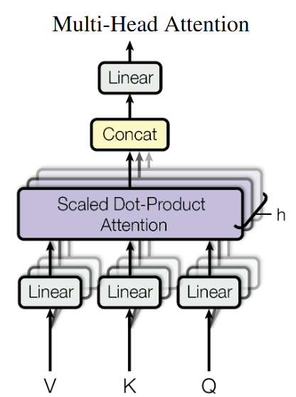
Multi-Head Attention: allows the model to jointly attend to information from different representation subspaces at different positions. With a single attention head, averaging inhibits this.
where \(\text{head}_i = \text{Attention}(QW_i^Q, KW_i^K, VW_i^V)\).
In this work we employ \(h=8\) parallel attention layers, or heads. For each of these we use \(d_k = d_v = d_{model}/h = 64\). Due to the reduced dimension of each head, the total computational cost is similar to that of single-head attention with full dimensionality.
classMultiHeadedAttention(nn.Module): def__init__(self, h, d_model, dropout=0.1): super(MultiHeadedAttention, self).__init__() assert d_model % h == 0 self.d_k = d_model // h self.h = h self.linears = clones(nn.Linear(d_model, d_model), 4) self.attn = None self.dropout = nn.Dropout(p=dropout) defforward(self, query, key, value, mask=None): if mask isnotNone: # Same mask applied to all h heads. mask = mask.unsqueeze(1) # shape from (batch_size, seq_len) to (batch_size, 1, seq_len) nbatches = query.size(0) # 1) Do all the linear projections in batch from d_model => h x d_k query, key, value = [l(x).view(nbatches, -1, self.h, self.d_k).transpose(1, 2) for l, x inzip(self.linears, (query, key, value))] # shape from (batch_size, seq_len, d_model) to (batch_size, h, seq_len, d_k) # 2) Apply attention on all the projected vectors in batch. x, self.attn = attention(query, key, value, mask=mask, dropout=self.dropout) # 3) "Concat" using a view and apply a final linear. x = x.transpose(1, 2).contiguous().view(nbatches, -1, self.h * self.d_k) del query, key, value returnself.linears[-1](x)
Applications of Attention in our Model
The Transformer uses multi-head attention in three different ways:
In “encoder-decoder attention” layers, the queries come from the previous decoder layer, and the memory keys and values come from the output of the encoder. This allows every position in the decoder to attend over all positions in the input sequence. This mimics the typical encoder-decoder attention mechanisms in sequence-to-sequence models such as (cite).
The encoder contains self-attention layers. In a self-attention layer all of the keys, values and queries come from the same place, in this case, the output of the previous layer in the encoder. Each position in the encoder can attend to all positions in the previous layer of the encoder.
Similarly, self-attention layers in the decoder allow each position in the decoder to attend to all positions in the decoder up to and including that position. We need to prevent leftward information flow in the decoder to preserve the auto-regressive property. We implement this inside of scaled dot-product attention by masking out (setting to \(-\infty\)) all values in the input of the softmax which correspond to illegal connections.
Position-wise Feed-Forward Networks
For the feed-forward MLP part: 2 layer FFN with a ReLU activation.
\[\text{FFN}(x)=\max(0, xW_1+b_1)W_2+b_2\]
Dimension: \(512\to 2048\to 512\).
Embeddings and Softmax
We use learned embeddings to convert the input tokens and output tokens to vectors of dimension \(d_{model}\). In the embedding layers, we multiply those weights by \(\sqrt{d_{model}}\). This results in the same effect as scaling the logits before the softmax, but we can share the weight matrix between the two embedding layers and the pre-softmax linear transformation, which makes training more efficient and reduces the number of parameters.
where \(pos\) is the position and \(i\) is the dimension. That is, each dimension of the positional encoding corresponds to a sinusoid. The wavelengths form a geometric progression from \(2\pi\) to \(10000\cdot 2\pi\). We chose this function because we hypothesized it would allow the model to easily learn to attend by relative positions, since for any fixed offset \(k\), \(PE_{pos+k}\) can be represented as a linear function of \(PE_{pos}\).
[!NOTE] Different from RoPE (where it uses a rotation matrix multiplying the query and key vectors), the original Transformer uses a fixed positional encoding added to the input embeddings. The RoPE method allows for better extrapolation to longer sequences and only depends on relative positions, while the original method is simpler and works well for many tasks.
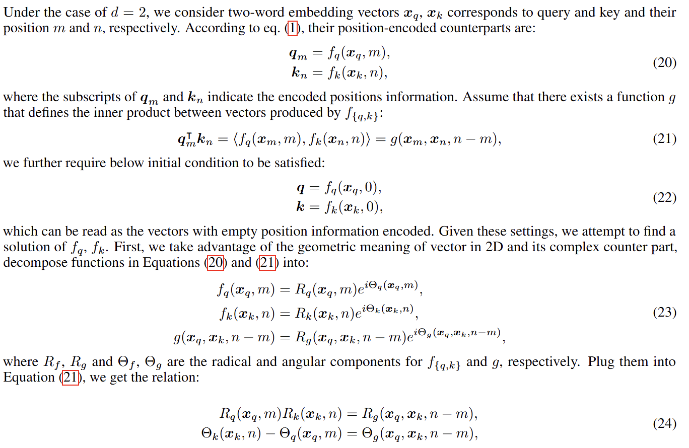
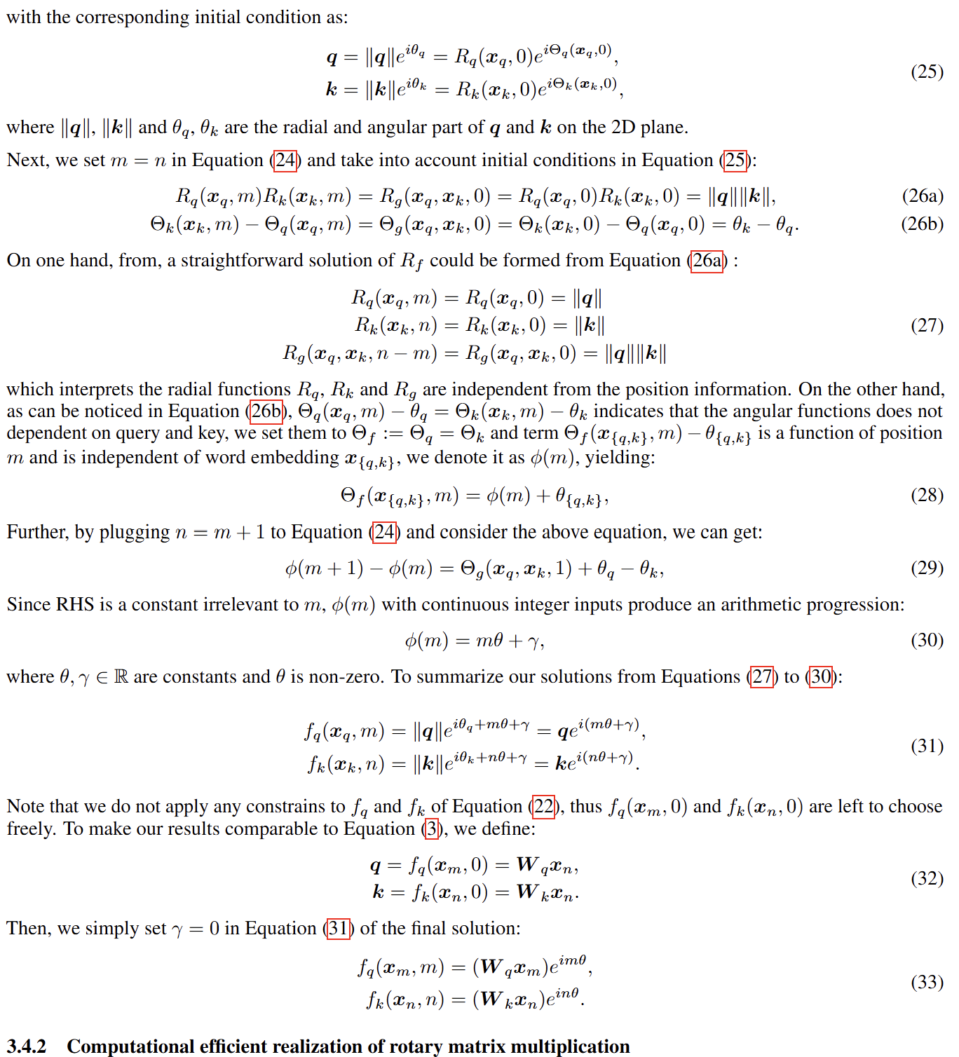
RoPE: Rotary Positional Embeddings.
Divide the \(d\)-dimensional space into \(d/2\) subspaces, and combine them in the merit of the linearity of the inner product, turning \(f_{q,k}\) into:
More Efficient Implementation: Since the rotation matrix is block diagonal and very sparse, we can implement it more efficiently than matrix multiplication:
where \(\otimes\) is the Hadamard product. This implementation is more efficient than matrix multiplication, and can be implemented in a few lines of code.
classPositionalEncoding(nn.Module): "Implement the PE function." def__init__(self, d_model, dropout, max_len=5000): super(PositionalEncoding, self).__init__() self.dropout = nn.Dropout(p=dropout) # Compute the positional encodings once in log space. pe = torch.zeros(max_len, d_model) position = torch.arange(0, max_len).unsqueeze(1) div_term = torch.exp(torch.arange(0, d_model, 2) * -(math.log(10000.0) / d_model)) pe[:, 0::2] = torch.sin(position * div_term) pe[:, 1::2] = torch.cos(position * div_term) pe = pe.unsqueeze(0) self.register_buffer('pe', pe) defforward(self, x): x = x + self.pe[:, :x.size(1)].requires_grad_(False) returnself.dropout(x)
# Extra exploration: use RoPE instead of sinusoidal positional encoding. # RoPE is a new positional encoding method that can be used in transformer models. # It is based on the idea of rotating the query and key vectors in the attention # mechanism, which allows the model to capture relative positional information # more effectively.
1 2 3 4 5 6 7 8 9 10 11 12 13 14 15 16 17 18 19
defmake_model(src_vocab, tgt_vocab, N=6, d_model=512, d_ff=2048, h=8, dropout=0.1): "Helper: Construct a model from hyperparameters." c = copy.deepcopy attn = MultiHeadedAttention(h, d_model) ff = PositionwiseFeedForward(d_model, d_ff, dropout) position = PositionalEncoding(d_model, dropout) model = EncoderDecoder( Encoder(EncoderLayer(d_model, c(attn), c(ff), dropout), N), Decoder(DecoderLayer(d_model, c(attn), c(attn), c(ff), dropout), N), nn.Sequential(Embeddings(d_model, src_vocab), c(position)), nn.Sequential(Embeddings(d_model, tgt_vocab), c(position)), Generator(d_model, tgt_vocab)) # This was important from their code. # Initialize parameters with Glorot / fan_avg. for p in model.parameters(): if p.dim() > 1: nn.init.xavier_uniform_(p) return model
Comments
Sign in with GitHub to join the conversation.